典型排序算法回顾
本文内容:
- 1.排序算法的分类
- 2.基于插入的排序
- 3.冒泡排序
- 4.快速排序
- 5.归并排序
- 6.选择排序
- 7.堆排序
1. 排序算法的分类
Sorting algorithms are often classified by: (Reference link)
- Computational complexity (worst, average and best behavior) in terms of the size of the list (n). For typical serial sorting algorithms good behavior is O(n log n), with parallel sort in O(log2 n), and bad behavior is O(n2). (See Big O notation.) Ideal behavior for a serial sort is O(n), but this is not possible in the average case. Optimal parallel sorting is O(log n). Comparison-based sorting algorithms, need at least O(n log n) comparisons for most inputs.
- Computational complexity of swaps (for “in-place” algorithms).
- Memory usage (and use of other computer resources). In particular, some sorting algorithms are “in-place”. Strictly, an in-place sort needs only O(1) memory beyond the items being sorted; sometimes O(log(n)) additional memory is considered “in-place”.
- Recursion. Some algorithms are either recursive or non-recursive, while others may be both (e.g., merge sort).
- Stability: stable sorting algorithms maintain the relative order of records with equal keys (i.e., values).
- Whether or not they are a comparison sort. A comparison sort examines the data only by comparing two elements with a comparison operator.
- General method: insertion, exchange, selection, merging, etc. Exchange sorts include bubble sort and quicksort. Selection sorts include shaker sort and heapsort. Also whether the algorithm is serial or parallel. The remainder of this discussion almost exclusively concentrates upon serial algorithms and assumes serial operation.
- Adaptability: Whether or not the presortedness of the input affects the running time. Algorithms that take this into account are known to be adaptive.
1.1 稳定性
排序算法的稳定性指的是,数组中相等元素在排序后,他们的相对位置不发生改变。
稳定排序算法的一个应用是:用第一和第二主键对数组进行排序。
比如对扑克牌,要求按数字大小进行排序,和按照花色进行排序(梅花、方块、红桃、黑桃),对于同一种花色,数字按照从小到大进行排序。第一轮按照数字从小到大进行排序(用任一种排序方法),第二轮用稳定的排序算法进行排序。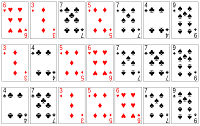
1.2 排序算法的比较

2. 基于插入的排序算法
2.1 直接插入排序
Insertion sort is a simple sorting algorithm that is relatively efficient for small lists and mostly sorted lists, and is often used as part of more sophisticated algorithms. It works by taking elements from the list one by one and inserting them in their correct position into a new sorted list.[17] In arrays, the new list and the remaining elements can share the array’s space, but insertion is expensive, requiring shifting all following elements over by one. Shell sort (see below) is a variant of insertion sort that is more efficient for larger lists.
It is much less efficient on large lists than more advanced algorithms such as quicksort, heapsort, or merge sort. However, insertion sort provides several advantages:
- Simple implementation: Bentley shows a three-line C version, and a five-line optimized version
- Efficient for (quite) small data sets, much like other quadratic sorting algorithms
- More efficient in practice than most other simple quadratic (i.e., O(n2)) algorithms such as selection sort or bubble sort
- Adaptive, i.e., efficient for data sets that are already substantially sorted: the time complexity is O(nk) when each element in the input is no more than k places away from its sorted position
- Stable; i.e., does not change the relative order of elements with equal keys
- In-place; i.e., only requires a constant amount O(1) of additional memory space
- Online; i.e., can sort a list as it receives it
| Worst case performance | О(n2) comparisons, swaps |
|---|---|
| Best case performance | O(n) comparisons, O(1) swaps |
| Average case performance | О(n2) comparisons, swaps |
| Worst case space complexity | О(n) total, O(1) auxiliary |
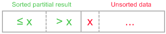
Insertion sort algorithm somewhat resembles selection sort. Array is imaginary divided into two parts - sorted one and unsorted one. At the beginning, sorted part contains first element of the array and unsorted one contains the rest. At every step, algorithm takes first element in the unsorted part and inserts it to the right place of the sorted one. When unsorted part becomes empty, algorithm stops. Sketchy, insertion sort algorithm step looks like this:
becomes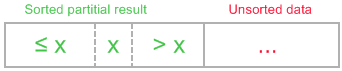

下面是插入排序的伪代码:(数组是从下标0开始的)
1 | INSERTION-SORT(A) |
C++语言实现(方法一:通过后移把元素放到正确的位置上):
1 | void insertion_sort(int A[], int n) { |
C++语言实现(方法二:通过交换把元素放到正确的位置上):
1 | void insertion_sort2(int A[], int n) { |
对链表的直接插入排序
If the items are stored in a linked list, then the list can be sorted with O(1) additional space. The algorithm starts with an initially empty (and therefore trivially sorted) list. The input items are taken off the list one at a time, and then inserted in the proper place in the sorted list. When the input list is empty, the sorted list has the desired result.
1 | struct LIST * SortList1(struct LIST * pList) |
The algorithm below uses a trailing pointer[6] for the insertion into the sorted list. A simpler recursive method rebuilds the list each time (rather than splicing) and can use O(n) stack space.
1 | struct LIST |
2.2 希尔排序
Shellsort, named after its inventor, Donald Shell, relies upon the fact that insertion sort does very well if the array is nearly sorted. Another way of saying this, is that insertion sort does well if it does not have to move each item “too far”. The idea is to repeatedly do insertion sort on all elements at fixed, decreasing distances apart:
1 | // 这里的数学公式 $h_k, h_{k-1}, ..., h_1=1$ |
The choice of increments turns out to be crucial. It turns out that a good choice of increments are these:
$h_1= 1, h_2= 3, h_3= 7, …, h_k= 2^k-1$
These increments are termed the Hibbard increments. The original increments suggested by the algorithm’s inventor were simple powers of 2, but the Hibbard increments do provably much better. To be able to use the $h_k$ increment, you need an array of size at least $h_k + 1$.
伪代码
The psuedo-code for shellSort using the Hibbard increments is as follows:
1 | find k0 so that 2^k0- 1 < size |
The fact that the last increment in the sequence is 1 means that regular insertion sort is done at the last step and therefore the array is guaranteed to be sorted by this procedure. The point is that when the increments are larger, there are fewer elements and they will be moved further than simply interchanging adjacent elements. At the last step, we do regular insertion sort and hopefully the array is “nearly sorted” which makes insertion sort come close to its best case behavior of running in linear time.
The notion that this is an speed improvement seems initially far-fetched. There are two enclosing for loops to get to an insertion sort, thus this algorithm has four enclosing loops.
希尔排序的C++代码实现
1 | void shell_sort(int A[], int n) |
ShellSort Analysis
Stability
Shellsort is not stable. It can be readily demonstrated with an array of size 4 (the smallest possible). Instability is to be expected because the increment-based sorts move elements distances without examining of elements in between.
Shellsort has O(n*log(n)) best case time
The best case, like insertion sort, is when the array is already sorted. Then the number of comparisons for each of the increment-based insertion sorts is the length of the array. Therefore we can determine:
comparisons =
n, for 1 sort with elements 1-apart (last step)
- 3 * n/3, for 3 sorts with elements 3-apart (next-to-last step)
- 7 * n/7, for 7 sorts with elements 7-apart
- 15 * n/15, for 15 sorts with elements 15-apart
- …
Each term is n. The question is how many terms are there? The number of terms is the value k such that
2^k - l < n
So k < log(n+1), meaning that the sorting time in the best case is less than n * log(n+1) = O(n*log(n)).
Shellsort worst case time is no worse than quadratic
The argument is similar as previous, but with a different overall computation.
comparisons ≤
n^2, for 1 sort with elements 1-apart (last step)
- 3 * (n/3)^2, for 3 sorts with elements 3-apart (next-to-last step)
- 7 * (n/7)^2, for 7 sorts with elements 7-apart
- 15 * (n/15)^2, for 15 sorts with elements 15-apart
- …
And so, with a bit of arithmetic, we can see that the number of comparisons is bounded by:
n^2 * (1 + 1/3 + 1/7 + 1/15 + 1/31 + …)
< n^2 * (1 + 1/2 + 1/4 + 1/8 + 1/16 + …)
= n^2 * 2
The last step uses the sum of the geometric series.
Shellsort worst and average times
The point about this algorithm is that the initial sorts, acting on elements at larger increments apart involve fewer elements, even considering a worst-case scenario. At these larger increments, “far-away” elements are swapped so that the number of inversions is dramatically reduced. At the later sorts of sorts at smaller increments, the behavior then comes closer to optimal behavior.
It can be proved that the worst-case time is sub-quadratic at $O(n^{3/2}) = O(n^{1.5}$
As can be expected, the proof is quite difficult. The textbook remarks that the average case time is unknown although conjectured to be $O(n^{5/4}) = O(n^{1.25})$
maybe it is (from wikipedia) $O(nlog^2n)$
The textbook also mentions other increment sequences which have been studied and seen to produce even better performance.
Reference Link: 希尔排序
3. 冒泡排序
Bubble sort, sometimes referred to as sinking sort, is a simple sorting algorithm that repeatedly steps through the list to be sorted, compares each pair of adjacent items and swaps them if they are in the wrong order. The pass through the list is repeated until no swaps are needed, which indicates that the list is sorted. The algorithm, which is a comparison sort, is named for the way smaller elements “bubble” to the top of the list. Although the algorithm is simple, it is too slow and impractical for most problems even when compared to insertion sort. It can be practical if the input is usually in sorted order but may occasionally have some out-of-order elements nearly in position.
注:正确的是顺序是小的在前,大的在后。
在输入规模较大时,冒泡排序的效率还不如插入排序,所以冒泡排序虽然简单,但是大多数时候并不使用它。
冒泡排序的演示如下图所示:
冒泡排序的C++实现:
1 | void bubble_sort(int A[], int n) |
对冒泡排序常见的改进方法是加入一标志性变量exchange,用于标志某一趟排序过程中是否有数据交换,如果进行某一趟排序时并没有进行数据交换,则说明数据已经按要求排列好,可立即结束排序,避免不必要的比较过程。设置一标志性变量pos,用于记录每趟排序中最后一次进行交换的位置。由于pos位置之后的记录均已交换到位,故在进行下一趟排序时只要扫描到pos位置即可。
冒泡排序的改进一:
1 | void bubble_sort2(int A[], int n) |
八大排序算法一文中,对冒泡排序算法做了另外的一种改进,如下代码所示,每一趟进行正反向的冒泡排序,同时找到最大值和最小值,不过我感觉此法并没有减少循环的次数。
1 | void bubble_sort3(int A[], int n) |
冒泡排序算法复杂度分析
| Data structure | Array |
|---|---|
| Best case performance | O(n) |
| Worst case performance | O(n^2) |
| Average case performance | О(n^2) |
| Worst case space complexity | O(1) auxiliary |
4. 快速排序
Quicksort (sometimes called partition-exchange sort) is an efficient sorting algorithm, serving as a systematic method for placing the elements of an array in order. Developed by Tony Hoare in 1959, with his work published in 1961, it is still a commonly used algorithm for sorting. When implemented well, it can be about two or three times faster than its main competitors, merge sort and heapsort.Quicksort
The quicksort algorithm is another classic divide and conquer algorithm. Unlike merge-sort, which does merging after solving the two subproblems, quicksort does all its work upfront.
Quicksort is a comparison sort, meaning that it can sort items of any type for which a “less-than” relation (formally, a total order) is defined. In efficient implementations it is not a stable sort, meaning that the relative order of equal sort items is not preserved. Quicksort can operate in-place on an array, requiring small additional amounts of memory to perform the sorting.
Mathematical analysis of quicksort shows that, on average, the algorithm takes O(n log n) comparisons to sort n items. In the worst case, it makes O(n^2) comparisons, though this behavior is rare.
4.1 快速排序的几种算法描述
4.1.1 快速排序的描述和Java代码实现(Open Data Structures(in Java))
Quicksort is simple to describe: Pick a random pivot element, x, from array A; partition A into the set of elements less than x, the set of elements equal to x, and the set of elements greater than x; and, finally, recursively sort the first and third sets in this partition. An example is shown in Figure.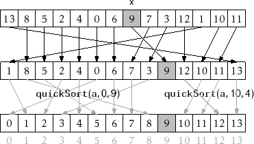
An example execution of quickSort(a,0,14,c)
Java代码实现:
1 | <T> void quickSort(T[] a, Comparator<T> c) { |
4.1.2 算法导论一书中第7章快速排序的描述
This scheme is attributed to Nico Lomuto and popularized by Bentley in his book Programming Pearls and Cormen et al. in their book Introduction to Algorithms. This scheme chooses a pivot which is typically the last element in the array. The algorithm maintains the index to put the pivot in variable i and each time it finds an element less than or equal to pivot, this index is incremented and that element would be placed before the pivot. As this scheme is more compact and easy to understand, it is frequently used in introductory material, although it is less efficient than Hoare’s original scheme. This scheme degrades to O(n^2) when the array is already sorted as well as when the array has all equal elements. There have been various variants proposed to boost performance including various ways to select pivot, deal with equal elements, use other sorting algorithms such as Insertion sort for small arrays and so on.
与归并排序一样,快速排序也使用了分治思想。下面是对一个典型的子数组A[p..r]进行快速排序的三步分治过程:
分解:数组A[p..r]被划分为两个(可能为空)子数组A[p..q-1]和A[q+1..r],使得A[p..q-1]中的每一个元素都小于等于A[q],而A[q]也小于等于A[q+1..r]中的每个元素。其中,计算下标q也是划分过程的一部分。
解决:通过递归调用快速排序,对子数组A[p..q-1]和A[q+1..r]进行排序。
合并:因为子数组都是原址排序的,所以不需要合并操作:数组A[p..r]已经有序。
假设数组的下标从0开始,算法的伪代码如下所示:
1 | QUICKSORT(A, p, r) |
在PARTITION的最后两行中,通过将主元与最左的大于x的元素进行交换,就可以将主元移动到它在数组中的正确位置上,并返回主元的新下标。PARTITION在子数组A[p..r]上的时间复杂度是O(n),其中n=r-p+1。
C++代码实现:
1 | /************************************************************************* |
注意
在讨论快速排序的平均性能时,我们假设输入序列的所有排列都是等概率的,这个假设并不总是成立,很多人都选择随机化版本的快速排序作为大数据输入情况下的排序算法。
在随机化的快速排序算法中,我们只需要在随机选择了枢轴元素后,把数组的最后一个元素和枢轴元素交换,这样的话我们就又可以利用上面的算法了。
4.1.3 Hoare partition scheme
The original partition scheme described by C.A.R. Hoare uses two indices that start at the ends of the array being partitioned, then move toward each other, until they detect an inversion: a pair of elements, one greater than the pivot, one smaller, that are in the wrong order relative to each other. The inverted elements are then swapped. When the indices meet, the algorithm stops and returns the final index. There are many variants of this algorithm, for example, selecting pivot from A[hi] instead of A[lo]. Hoare’s scheme is more efficient than Lomuto’s partition scheme because it does three times fewer swaps on average, and it creates efficient partitions even when all values are equal. Like Lomuto’s partition scheme, Hoare partitioning also causes Quicksort to degrade to O(n^2) when the input array is already sorted; it also doesn’t produce a stable sort. Note that in this scheme, the pivot’s final location is not necessarily at the index that was returned, and the next two segments that the main algorithm recurs on are [lo..p] and (p..hi] as opposed to [lo..p) and (p..hi] as in Lomuto’s scheme. In pseudocode,
1 | algorithm quicksort(A, lo, hi) is |
C++代码实现:
1 | class QuickSort { |
注意
上面提到的 Hoare partition scheme 和 Lomuto partition scheme 的算法在改变了枢轴元素的位置后,算法的代码要做相应的改变,比较简单的做法是,像快排的随机化版本那样,交换枢轴元素到第一个或最后一个元素的位置处。下面是 Hoare partition scheme 算法的一个变体,该算法较易明白,而且用元素的赋值代替了交换操作,如果取枢轴元素为最后一个的话,需要先从low考虑小于枢轴元素的情况,再从high考虑大于枢轴元素的情况。如果取枢轴元素为第一个的话,需要先从high考虑大于枢轴元素的情况,再从low考虑小于枢轴元素的情况。
算法的C++实现:
1 | void quick_sort(int A[], int left, int right) |
4.2 快速排序的算法复杂度分析
| Data structure | Array |
|---|---|
| Best case performance | O(n log n) (simple partition) or O(n) (three-way partition and equal keys) |
| Worst case performance | O(n^2) |
| Average case performance | O(n log n) |
| Worst case space complexity | O(n) auxiliary (naive), O(log n) auxiliary (Sedgewick 1978) |
5. 归并排序
Definition: A sort algorithm that splits the items to be sorted into two groups, recursively sorts each group, and merges them into a final, sorted sequence. Run time is Θ(n log n).
Conceptually, a merge sort works as follows:
1) Divide the unsorted list into n sublists, each containing 1 element (a list of 1 element is considered sorted).
2) Repeatedly merge sublists to produce new sorted sublists until there is only 1 sublist remaining. This will be the sorted list.
5.1 算法的伪代码描述
归并排序的的关键是合并两个已经排好序的数组,假设子数组A[p ... q]和A[q+1 ... r]已经排好序,下面的算法是合并这两个子数组及归并排序。
这里的伪代码为算法导论一书中的归并排序算法改进而来。
1 | MERGE(A, p, q, r) |
维基百科中对归并排序的算法实现:
Top-down implementation
Example C-like code using indices for top down merge sort algorithm that recursively splits the list (called runs in this example) into sublists until sublist size is 1, then merges those sublists to produce a sorted list. The copy back step could be avoided if the recursion alternated between two functions so that the direction of the merge corresponds with the level of recursion.
1 | // Array A[] has the items to sort; array B[] is a work array. |
Bottom-up implementation
Example C-like code using indices for bottom up merge sort algorithm which treats the list as an array of n sublists (called runs in this example) of size 1, and iteratively merges sub-lists back and forth between two buffers:
1 | // array A[] has the items to sort; array B[] is a work array |
Top-down implementation using lists
Pseudocode for top down merge sort algorithm which recursively divides the input list into smaller sublists until the sublists are trivially sorted, and then merges the sublists while returning up the call chain.
1 | function merge_sort(list m) |
In this example, the merge function merges the left and right sublists.
1 | function merge(left, right) |
Bottom-up implementation using lists
Pseudocode for bottom up merge sort algorithm which uses a small fixed size array of references to nodes, where array[i] is either a reference to a list of size 2^i or 0. node is a reference or pointer to a node. The merge() function would be similar to the one shown in the top down merge lists example, it merges two already sorted lists, and handles empty lists. In this case, merge() would use node for its input parameters and return value.
1 | function merge_sort(node head) |
5.2 算法复杂度分析
| Data structure | Array |
|---|---|
| Best case performance | O(n log n) typical, O(n) natural variant |
| Worst case performance | O(n log n) |
| Average case performance | O(n log n) |
| Worst case space complexity | О(n) total, O(n) auxiliary |
5.3 和其他排序算法的比较:
Although heapsort has the same time bounds as merge sort, it requires only Θ(1) auxiliary space instead of merge sort’s Θ(n). On typical modern architectures, efficient quicksort implementations generally outperform mergesort for sorting RAM-based arrays.[citation needed] On the other hand, merge sort is a stable sort and is more efficient at handling slow-to-access sequential media. Merge sort is often the best choice for sorting a linked list: in this situation it is relatively easy to implement a merge sort in such a way that it requires only Θ(1) extra space, and the slow random-access performance of a linked list makes some other algorithms (such as quicksort) perform poorly, and others (such as heapsort) completely impossible.
As of Perl 5.8, merge sort is its default sorting algorithm (it was quicksort in previous versions of Perl). In Java, the Arrays.sort() methods use merge sort or a tuned quicksort depending on the datatypes and for implementation efficiency switch to insertion sort when fewer than seven array elements are being sorted. Python uses Timsort, another tuned hybrid of merge sort and insertion sort, that has become the standard sort algorithm in Java SE 7, on the Android platform, and in GNU Octave.
5.4 归并排序图例演示

5.5 对链表归并排序的示例
合并两个有序的链表
要求:使用常量的额外空间
1 | /********************************************************************************** |
使用归并排序对链表进行排序
方法一
1 | /** |
方法二
1 | /********************************************************************************** |
6. 选择排序
In computer science, selection sort is a sorting algorithm, specifically an in-place comparison sort. It has O(n^2) time complexity, making it inefficient on large lists, and generally performs worse than the similar insertion sort. Selection sort is noted for its simplicity, and it has performance advantages over more complicated algorithms in certain situations, particularly where auxiliary memory is limited.
The algorithm divides the input list into two parts: the sublist of items already sorted, which is built up from left to right at the front (left) of the list, and the sublist of items remaining to be sorted that occupy the rest of the list. Initially, the sorted sublist is empty and the unsorted sublist is the entire input list. The algorithm proceeds by finding the smallest (or largest, depending on sorting order) element in the unsorted sublist, exchanging (swapping) it with the leftmost unsorted element (putting it in sorted order), and moving the sublist boundaries one element to the right.
6.1 实现
1 | /* a[0] to a[n-1] is the array to sort */ |
6.2 分析
Selection sort is not difficult to analyze compared to other sorting algorithms since none of the loops depend on the data in the array. Selecting the lowest element requires scanning all n elements (this takes n − 1 comparisons) and then swapping it into the first position. Finding the next lowest element requires scanning the remaining n − 1 elements and so on, for (n − 1) + (n − 2) + … + 2 + 1 = n(n - 1) / 2 ∈ Θ(n^2) comparisons (see arithmetic progression).[1] Each of these scans requires one swap for n − 1 elements (the final element is already in place).
6.3 选择排序演示
Selection sort animation. Red is current min. Yellow is sorted list. Blue is current item.
7. 堆排序
In computer science, heapsort is a comparison-based sorting algorithm. Heapsort can be thought of as an improved selection sort: like that algorithm, it divides its input into a sorted and an unsorted region, and it iteratively shrinks the unsorted region by extracting the largest element and moving that to the sorted region. The improvement consists of the use of a heap data structure rather than a linear-time search to find the maximum.
Although somewhat slower in practice on most machines than a well-implemented quicksort, it has the advantage of a more favorable worst-case O(n log n) runtime. Heapsort is an in-place algorithm, but it is not a stable sort.
The heapsort algorithm can be divided into two parts.
In the first step, a heap is built out of the data. The heap is often placed in an array with the layout of a complete binary tree. The complete binary tree maps the binary tree structure into the array indices; each array index represents a node; the index of the node’s parent, left child branch, or right child branch are simple expressions. For a zero-based array, the root node is stored at index 0; if i is the index of the current node, then
1 | iParent(i) = floor((i-1) / 2) |
In the second step, a sorted array is created by repeatedly removing the largest element from the heap (the root of the heap), and inserting it into the array. The heap is updated after each removal to maintain the heap. Once all objects have been removed from the heap, the result is a sorted array.
Heapsort can be performed in place. The array can be split into two parts, the sorted array and the heap. The storage of heaps as arrays is diagrammed here. The heap’s invariant is preserved after each extraction, so the only cost is that of extraction.
7.1 实现
(参考算法导论第3版堆排序一章并有所修改)
二叉堆有两种,最大堆和最小堆(小根堆)。在最大堆中,最大堆的特性是指除了根以外的每个节点i,有A[PARENT(i)] >= A[i],这样在最大堆中最大的元素在树的根部。最小堆则相反,最小堆的特性是除了根节点以外的每个节点i,有A[PARENT(i)] <= A[i],这样在最小堆中最小的元素在树的根部。
堆排序的过程:
buildMaxHeap()过程,以O(n)时间运行,可以在无序的输入数组基础上构建出最大堆。- 交换数组中的第一个元素和最后一个元素,数组中的最大元素被移动到了它的最终位置,待排序的数组长度减少了1.
- 调用
maxHeapify()过程,保持最大堆的性质,使最大的元素在堆的根部,此步骤的时间复杂度是O(log(n))。 - 重复步骤2直到未排序的数组中的元素个数减少到1。
算法的伪代码如下:
maxHeapify()是用于维护堆的性质,它的输入为一个数组A和一个下标i,在调用maxHeapify()的时候,我们假定根节点为iLeftChild(i)和iRightChild(i)的二叉树都是最大堆,但这时A[i]有可能小于其孩子,这样就违背了最大堆的性质。maxHeapify()通过让A[i]的值在最大堆中“逐级下降”,从而使得以下标i为根节点的子树重新遵循最大堆的性质。
1 | maxHeapify(A, i) { |
对于一棵以i为根节点,大小为n的子树,maxHeapify()的时间代价包括:调整A[i]和A[iLeftChild(i)]和A[iRightChild(i)]的关系的时间代价Θ(1),加上在一棵以i的一个孩子为根节点的子树上运行maxHeapify()的时间代价(这里假设递归调用会发生)。因为每个孩子的子树的大小至多为2n/3(最坏情况发生在树的最底层恰好半满的时候),可以用下面的递归式表达运行时间:
$T(n) \leq T(2n/3)+\Theta(1)$
根据主定理,上述递归式的解为O(logn)。
假设数组的长度为n,则子数组A[(n-1-1)/2+1...n-1]中的元素都是树的叶子节点,每个叶子节点都可以看成只包含一个元素的堆。过程buildMaxHeap()对树中的其他节点都调用一次maxHeapify()。这是一个自底向上的建堆过程。
1 | buildMaxHeap(A) { |
堆排序算法:
1 | heapSort(A) { |
7.2 和其他排序算法的比较(Comparison with other sorts)
Heapsort primarily competes with quicksort, another very efficient general purpose nearly-in-place comparison-based sort algorithm.
Quicksort is typically somewhat faster due to some factors, but the worst-case running time for quicksort is O(n^2), which is unacceptable for large data sets and can be deliberately triggered given enough knowledge of the implementation, creating a security risk. See quicksort for a detailed discussion of this problem and possible solutions.
Thus, because of the O(n log n) upper bound on heapsort’s running time and constant upper bound on its auxiliary storage, embedded systems with real-time constraints or systems concerned with security often use heapsort.
Heapsort also competes with merge sort, which has the same time bounds. Merge sort requires Ω(n) auxiliary space, but heapsort requires only a constant amount. Heapsort typically runs faster in practice on machines with small or slow data caches, and does not require as much external memory. On the other hand, merge sort has several advantages over heapsort:
- Merge sort on arrays has considerably better data cache performance, often outperforming heapsort on modern desktop computers because merge sort frequently accesses contiguous memory locations (good locality of reference); heapsort references are spread throughout the heap.
- Heapsort is not a stable sort; merge sort is stable.
- Merge sort parallelizes well and can achieve close to linear speedup with a trivial implementation; heapsort is not an obvious candidate for a parallel algorithm.
- Merge sort can be adapted to operate on singly linked lists with O(1) extra space. Heapsort can be adapted to operate on doubly linked lists with only O(1) extra space overhead.
- Merge sort is used in external sorting; heapsort is not. Locality of reference is the issue.
Introsort is an alternative to heapsort that combines quicksort and heapsort to retain advantages of both: worst case speed of heapsort and average speed of quicksort.
7.3 算法复杂度分析
| Data structure | Array |
|---|---|
| Best case performance | O(n log n), Ω(n) |
| Worst case performance | O(n log n) |
| Average case performance | O(n log n) |
| Worst case space complexity | O(1) auxiliary |
7.4 堆排序演示

7.5 堆排序的C++代码实现
1 |
|
Reference Links:
九大排序算法再总结
九大基础排序总结与对比
数据结构复习之【排序】
八大排序算法
Sorting algorithm
希尔排序
排序算法视频演示:
http://www.bilibili.com/video/av685670/
http://airtucha.github.io/SortVis/